HOW TO RANK AND GRADE STUDENT MARKS WITH EXCEL OR GOOGLE SHEETS. SIMPLE FORMULAE AND FUNCTIONS

Ranking and grading student marks can sometimes be a tedious and confusing work given the formulae and functions involved. In this this manual, we will illustrate to you how to achieve this.

Consider the Mathematics grading system  below:

Mathematics Grading System

• 0 - 24       E
• 25 - 29     D-
• 30 - 34     D
• 35 - 39     D+
• 40 - 44     C-
• 45 - 49     C
• 50 - 54     C+
• 55 - 59     B-
• ​60 - 64     B
• 65 - 69     B+
• 70 - 74     A-
• 75 - 100   A

BASIC FUNCTIONS AND FORMULA IN EXCEL/SHEETS USED FOR GRADING

USING THE 'NESTED IF' FORMULA

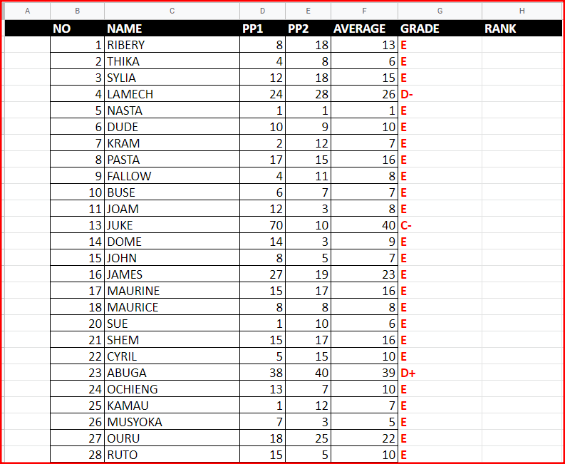
Consider the Excel sheet below

open/download in excel sheet

To grade the average column, we will put this nested if formula in cell G2 and copy it downwards

​=IF(F2>=75,"A",IF(F2>=70,"A-", IF(F2>=65,"B+",IF(F2>=60,"B",IF(F2>=55,"B-",IF(F2>=50,"C+",IF(F2>=45,"C",IF(F2>=40,"C-",IF(F2>=35,"D+",IF(F2>=30,"D",IF(F2>=25,"D-","E")))))))))))

using the formula above, we get this result

Sometimes, the above function may give wrong grades due to rounding  errors.
In rounding errors for example, a number such as 29.5 may be rounded off to 30 by the computer as instructed by the user. The user will see 30 but the computer will see 29.5 hence giving grades contrary to the users expectation. When such a challenge happens, use this formula.

Note: the formula references values in cell f3

​=IF(F3>=74.5,"A",IF(F3>=69.5,"A-", IF(F3>=64.5,"B+",IF(F3>=59.5,"B",IF(F3>=54.5,"B-",IF(F3>=49.5,"C+",IF(F3>=44.5,"C",IF(F3>=39.5,"C-",IF(F3>=34.5,"D+",IF(F3>=29.5,"D",IF(F3>=24.5,"D-","E")))))))))))

---

---

try it yourself

---

Using the ranking formula

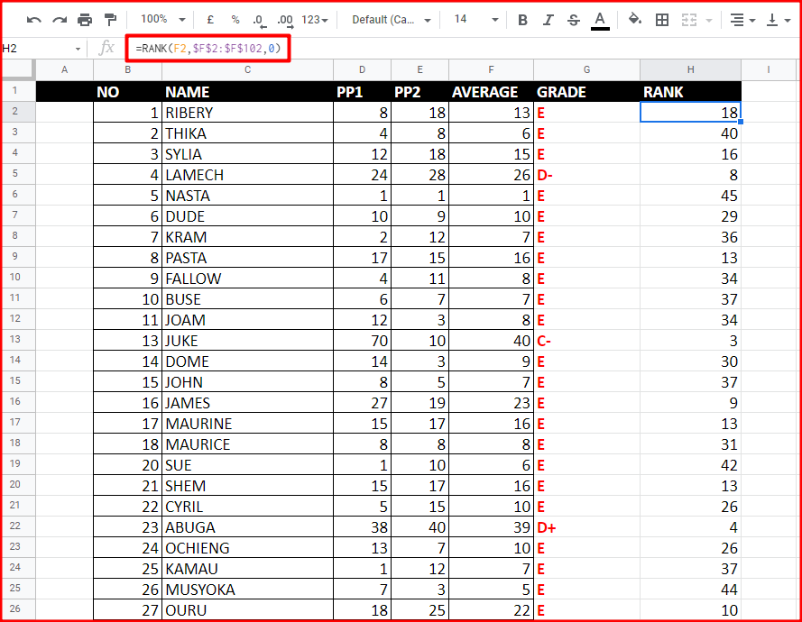
Paste this ranking formula in cell H2 

​=RANK(F2,$F$2:$F$102,0)

here is the outcome

---

---

To arrange students according to their performance, use the sort command on average column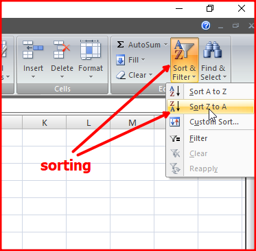

1. highlight all the values in the average column
2. Locate sort and filter control of the ribbon
3. sort z to a or in descending order for the best performing student to start from above.

I hope that you got the answers you were seeking. just incase you have any question in this excel topic, feel free to ask it in the comment section below.